Excel/VBA with Rubberduck
Excel/VBA Examples
This page provides practical Excel and VBA examples, including advanced formulas, pivot tables, charting, and automation. The focus is on real-world actuarial and business use cases, with interactive tables and annotated code.
Key topics covered:
| Topic | Description |
|---|---|
| Conditional Formatting | Highlighting data based on rules |
| Advanced Formulas | Efficient data processing and analysis |
| Pivot Tables | Summarizing and visualizing data |
| Graphs/Charting | Visual representation of data |
| VLOOKUP/Index-Match | Data lookup and retrieval |
Sample Problem
"What is the total average cost of the following claims?"
| Accident Year | Amount of Each Claim | Number of Claims |
|---|---|---|
| 1998 | $6,000 | 5 |
| 2005 | $10,000 | 3 |
| 2010 | $20,000 | 2 |
Add a total for each year:
| Accident Year | Amount of Each Claim | Number of Claims | Total |
|---|---|---|---|
| 1998 | $6,000 | 5 | $30,000 |
| 2005 | $10,000 | 3 | $30,000 |
| 2010 | $20,000 | 2 | $40,000 |
This is a straightforward application of the weighted average formula, where the expected value E(X) is calculated as the total claims divided by the number of claims.
Next: "If the claim costs rise at an annual rate of 15% since 2009 and 10% in prior years, what will the average cost be in 2012?"
Replicating a Spreadsheet with Advanced Formulas
The objective is to maximize the use of built-in Excel functions to efficiently process and analyze data.
The data below is presented in a static HTML table for clarity and ease of review.
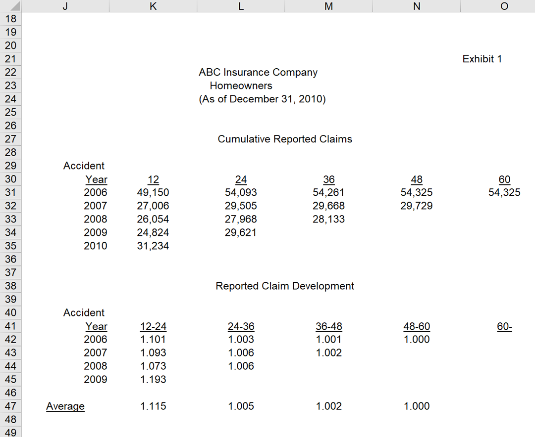
Cumulative Reported Claim
| Accident Year | 12 | 24 | 36 | 48 | 60 |
|---|---|---|---|---|---|
| 2006 | $49,150 | $54,093 | $54,261 | $54,325 | $54,325 |
| 2007 | $49,150 | $54,093 | $54,261 | $54,325 | |
| 2008 | $49,150 | $54,093 | $54,261 | ||
| 2009 | $49,150 | $54,093 | |||
| 2010 | $31,234 |
Reported Claim Development
| Accident Year | 12-24 | 24-36 | 36-48 | 48-60 | 60-Ult |
|---|---|---|---|---|---|
| 2006 | 1.101 | 1.003 | 1.001 | 1 | |
| 2007 | 1.093 | 1.006 | 1.002 | ||
| 2008 | 1.073 | 1.006 | |||
| 2009 | 1.193 | ||||
| Average | 1.115 | 1.005 | 1.002 | 1 |

The relationship between Cumulative Reported Claims and Reported Claim Development is determined by dividing the value at time t+1 by the value at time t. The IFERROR function in Excel is used to handle errors such as division by zero:
=IFERROR(value, value_if_error)For example, to safely divide two cells and return a blank if an error occurs:
=IFERROR(L34/K34,"")This approach ensures that the resulting tables are both accurate and user-friendly, supporting robust data analysis and reporting.
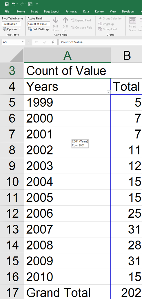
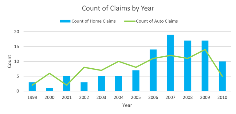
Pivot Table Analysis
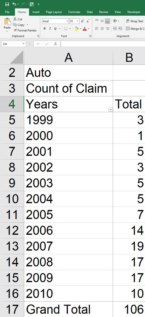
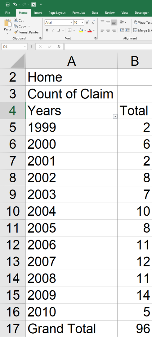
Combine results from both tables for a total:
| Year | Number of Claims (Auto + Home) |
|---|---|
| 1999 | 5 |
| 2000 | 7 |
| 2001 | 7 |
| 2002 | 11 |
| 2003 | 12 |
| 2004 | 15 |
| 2005 | 15 |
| 2006 | 25 |
| 2007 | 31 |
| 2008 | 28 |
| 2009 | 31 |
| 2010 | 15 |
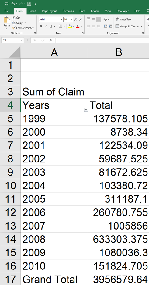
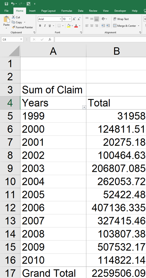
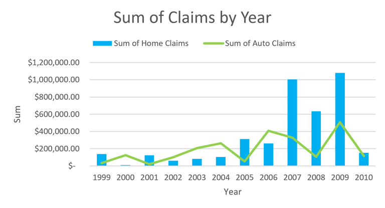
Total Cost of Claims by Occurrence Year
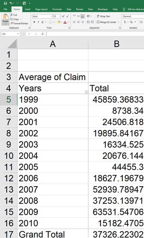
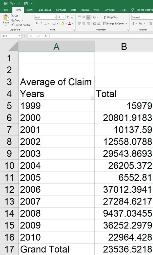
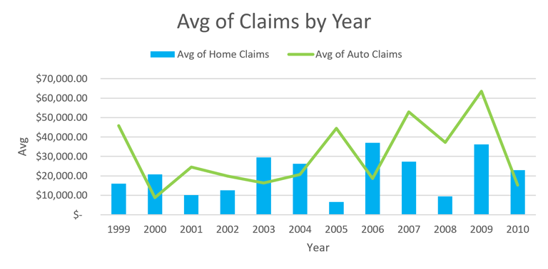
Average Cost of Claim by Occurrence Year
Graphs/Advanced Charting Techniques
VLOOKUP Function
=VLOOKUP(value, table, col_index, [range_lookup])
value: The search query.
table: The table or range.
col_index: The column index to return.
range_lookup: 1 (approximate) or 0 (exact match).
Note: VLOOKUP cannot search to the left of the lookup column. For more flexibility and efficiency, use INDEX-MATCH.
INDEX-MATCH Example:
=INDEX(return_range, MATCH(lookup_value, lookup_range, 0))This approach is more efficient for large datasets and allows for flexible lookups in any direction.
Contact: trejo.juann@gmail.com